
In communications, signal propagation theory studies the movement of signals from the transmitter to the receiver through a transmission medium. Depending on the characteristics of the signal and the medium, different situations may arise. In general, the cases are classified according to the type of distortion they produce in the transmitted signal.
This text is structured with the following table of contents:
1. Signal Propagation Introduction
This article explains, both conceptually and with motion graphics, the most typical cases that occur in signal propagation. For a correct understanding of the text it is necessary to review the following concepts, thoroughly explained in previous articles:
- Waves and Wavemotion: waves are the sinusoidal disturbances that make up a signal.
- Phase Velocity: propagation velocity of any of the phases of a sinusoid.
- Group Velocity: propagation velocity of the envelope of a modulated carrier.
It is important to emphasize that this text focuses on the simple propagation, along a single path, of a signal through a medium between transmitter and receiver. In other words, for the sake of simplicity, other phenomena such as multiple paths or reflections are not taken into account.
2. Fundamental Factors in Signal Propagation
The different cases of signal propagation are derived from two fundamental factors: the spectrum of the signal to transmit [1] and the physical parameters of the transmission medium. [2].
2.1 Signal Spectrum
From the point of view of signal propagation, there are two types of signals: baseband and passband.
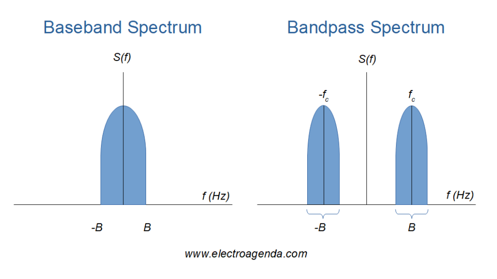
2.1.1 Base Band Signal
A baseband signal is transmitted over the transmission medium as originally generated, without modulating a carrier. In that sense, the signal is composed of frequency components that can range from DC to the signal bandwidth, B in the Figure above (left).
This case is easier to analyze because there is no group or envelope that can move at a speed different from that of the overall signal.
2.1.2 Band Pass Signal
Bandpass signals are created when a modulating or envelope signal (typically a baseband signal) modulates a carrier. Consequently the frequency components of the bandpass signal are bounded by a bandwidth B around a center frequency, that of the carrier, as shown in the Figure above (right).
Unlike the baseband signal, in a bandpass signal the group velocity of the envelope and the phase velocity of the overall signal can be different. This results in more complexity and more cases in terms of propagation.
2.2 Physical Parameters of the Transmission Medium
2.2.1 Refractive Index
The propagation or phase velocity vp of a wave depends on the refractive index n of the transmission medium. Additionally, the n value depends on multiple factors such as frequency ω, density, temperature or even the direction of propagation. [2].
In general, for given conditions, the phase velocity can be represented as a function of the frequency-dependent refractive index:
\begin{equation} v_p(\omega) = \frac{c}{n(\omega)} \end{equation}
Where c represents the speed of light.
2.2.2 Signal Propagation Function in the Medium
In practice, for the established conditions a function ω(k), or k(ω), can be derived, which determines the characteristics of the signal propagation through the medium.
Recall that ω represents the frequency of the wave and k its propagation constant or wave number, as explained in this link. Often the propagation constant is also represented by the symbol β.
Moreover, the phase velocity vp is dependent on ω and k according to the following equation:
\begin{equation} v_p(\omega) = \frac{\omega}{k(\omega)} \end{equation}
Therefore, by comparing the phase velocity of equations (1) and (2) the function k(ω) can be obtained from n(ω):
\begin{equation} k(\omega) = \frac{\omega · n(\omega)}{c} \end{equation}
Finally, the group velocity vg can also be derived for any frequency from the above function k(ω):
\begin{equation} v_g(\omega) = \frac{1}{\cfrac{\partial k(\omega)}{\partial \omega}} \end{equation}
2.2.3 Signal Propagation Polynomial
Using Taylor series, the function k(ω) can be approximated by a polynomial in the signal bandwidth (a similar exercise was performed in this link). Simplifying, the most typical cases of signal propagation can be analyzed using a generic second-order polynomial:
\begin{equation} k(\omega) = a_2\omega^2 + a_1\omega+a_0 \end{equation}
Note that the above equation is a simplification of reality to explain signal propagation in a simple and generic way. For a more detailed analysis, the mathematics of more complex cases, such as fiber optic propagation, can be consulted [3].
3. Signal Propagation Case Classification
This section classifies the different cases of signal propagation that will later be shown in motion in section 4. As a starting point, a generic propagation equation is obtained from which the different cases can be analyzed, which are then synthesized in a summary table.
3.1 Generic Signal Propagation Equation
We start from a generic signal to be transmitted at the origin (x=0). Each component of the signal is characterized by a frequency ω, its amplitude Ai and its phase φi. Thus the signal can be written as follows:
\begin{equation} s_{tx}(t) = \sum_iA_i \cos(\omega_i t + \varphi_i) \end{equation}
The signal received at the receiver, located at position x, will be given by the following expression:
\begin{equation} s_{rx}(t,x) = \sum_iA_i \cos[\omega_i t - k(\omega)x + \varphi_i] \end{equation}
Substituting k(ω) into expression (5) gives:
\begin{equation} s_{rx}(t,x) = \sum_iA_i \cos[\omega_i( t - a_2\omega_i x - a_1x) - a_0x + \varphi_i] \end{equation}
3.2 Signal Propagation Summary Table
From the above equation, depending on whether or not the values of a2, a1 and a0 are equal to zero, different cases can occur, which are summarized in the following table. The calculations are also supported by equation (2) of the phase velocity and equation (4) of the group velocity.
| a_2 | a_1 | a_0 | v_p | v_g | Baseband Signal | Passband Signal | Comments | Links |
|---|---|---|---|---|---|---|---|---|
| (0) | (≠0) | (0) | \cfrac{1}{a_1} | \cfrac{1}{a_1} | Delay. | Delay. | Linear Phase Shift. No distortion. | 4.1 |
| (0) | (≠0) | (≠0) | \cfrac{1}{a_1+\cfrac{a_0}{\omega}} | \cfrac{1}{a_1} | Distortion. | Signal Distortion. Undistorted envelope. | Frequency Constant Phase Shift. | 4.2 |
| (≠0) | (≠0) | (0) | \cfrac{1}{a_2\omega+a_1} | \cfrac{1}{2a_2\omega+a_1} | Distortion. | Distortion. | Dispersion. | 4.3 |
| (≠0) | (≠0) | (≠0) | \cfrac{1}{a_2\omega+a_1+\cfrac{a_0}{\omega}} | \cfrac{1}{2a_2\omega+a_1} | Distortion. | Distortion. | Dispersion. (+Constant Phase Shift). | 4.4 |
| (x) | (0) | (x) | – | – | – | – | No propagation. | 4.5 |
The “Link” column contains links to the corresponding sections where moving signals are displayed.
As a summary, it can be stated that:
- The constant a0 introduces constant phase shifts in frequency. For baseband signals they imply distortion, while for bandpass signals they do not imply distortion in the demodulated signal.
- The constant a1 introduces linear phase shift with frequency, which only results in a delay of the transmitted signal.
- The constant a2 introduces distortion in the signal, also in the demodulated signal, usually called dispersion.
4. Examples of Signal Propagation in Motion
Moving examples of all the cases explained are shown below. In all of them Gaussian pulses are used as baseband signal.
4.1 Signal Propagation with Linear Phase Shift
In this case both the phase velocity and the group velocity of all the frequency components of the signal are the same, regardless of the frequency. Therefore, during propagation, the signal is shifted without changing its shape. In other words, the original signal arrives at the receiver with a delay but without distortion.
4.1.1 Baseband Signal Propagation with Linear Phase Shift
This case is shown below in motion for a baseband pulse:

The pulse maintains its original shape throughout the displacement.
4.1.2 Bandpass Signal Propagation with Linear Phase Shift
The following graph illustrates the equivalent case for a bandpass pulse, i.e. a pulse modulating a carrier:

It can be seen that both the envelope and the signal move at the same speed, without distortion.
4.2 Constant Frequency Phase Shift Signal Propagation
In this case, during signal propagation, in addition to the linear phase shift that results in the corresponding delay, a constant phase shift is added, equal for all frequencies. This phenomenon is discussed in detail in this link.
To summarize, phase velocity and group velocity are different, as shown in the summary table. While the phase velocity is frequency dependent, which causes distortion in the propagating signal, the group velocity is constant, so the envelope remains unchanged during its displacement.
4.2.1 Constant Phase Shift Baseband Signal Propagation
The phenomenon described above translates into distortion for a baseband signal, as illustrated below:

Note that in the example shown the phase shift is constant in frequency but dependent on the x position. The video signal ends with a phase shift of -90º (at the x=2m position), equivalent to a Hilbert Transform.
4.2.2 Bandpass Signal Propagation with Constant Phase Shift
However, for a bandpass signal, the signal changes its appearance as in the previous example, but the envelope is not distorted as shown below:
In this way there is no distortion in the demodulated signal, which is the one that was really intended to be communicated and which coincides with the envelope.
Note that despite the dependence of phase velocity on frequency, the overall signal as a whole propagates at the carrier phase velocity, as demonstrated here and here.
4.3 Signal Propagation with Dispersion
In dispersive transmission media both the phase velocity and the group velocity are frequency dependent. Thus both the signal and the envelope are distorted during propagation.
Typically, dispersion is a phenomenon that appears in bandpass signals. In particular, the most significant case of communications with dispersion is fiber optic propagation [3]. However, for the sake of completeness, this section also shows examples of baseband signals to which dispersion is applied.
4.3.1 Baseband Signal Propagation with Dispersion
In line with the above, the following image illustrates a baseband pulse that disperses during its propagation:

It is observed that the baseband pulse is greatly distorted during propagation due to the different velocity of its frequency components.
4.3.2 Bandpass Signal Propagation with Dispersion
The most characteristic case of propagation with dispersion, namely a bandpass Gaussian pulse, is shown below:

The blue signal represents the propagation of the bandpass Gaussian pulse. On the other hand, the red signal represents the envelope of the original Gaussian pulse, before applying dispersion. This undistorted envelope is shifted along with the bandpass signal to make the dispersion effect easier to visualize.
The video shows how the bandpass pulse progressively widens during propagation, while the maximum amplitude decreases. It can be concluded that the term “dispersion” is coined because the pulse energy is dispersed during propagation, i.e., the pulse progressively occupies a larger time interval.
4.3.3 Effects on Communications
In the above example, the demodulated signal at the receiver would be the envelope of the pulse affected by the dispersion. In other words, dispersion is associated with a broadening of the transmitted signal. The example with pulses illustrates very well how dispersion adversely affects communications.
Indeed, if the pulse represents the binary ‘1’ and the absence of pulse represents the binary ‘0’, the widening associated with the dispersion can translate into errors when detecting contiguous bits, as shown in the following video:

This phenomenon typically occurs in fiber optic communications, with dispersion being one of the most limiting factors in the capacity and length of a link [3].
4.4 Signal Propagation with Dispersion and Constant Phase Shift
For the baseband case, by adding a constant phase shift (a0) in addition to the dispersion (a2), an effect equivalent to the sum of both phenomena can be seen. However, as mentioned above, this is not a very representative case for any real communications medium.
On the other hand, for the case of bandpass dispersion, as in an optical fiber, the constant phase shift (a0) is also part of the propagation constant together with the dispersion (a2). However, the effect of the constant phase shift is not very significant, since it has no influence on the pulse envelope, being dispersion the most noticeable effect.
Therefore, the images and videos in the previous sections are already sufficiently representative to visualize this case. Consequently, no further images are added in this section.
4.5 No Propagation Case
Note that any situation where a1 equals zero implies that the signal does not move in time, which makes no physical sense from the propagation point of view.
5. Conclusions
The main conclusions of this article are as follows:
- The propagation of a signal through a transmission medium is determined by the signal spectrum and the parameters of the medium.
- The transmission medium has a function k(ω) associated with it from which the effects on the signal during propagation can be derived.
- For a function k(ω)=a2ω2+a1ω+a0 , the constant a0 implies a constant phase shift in frequency, the constant a1 produces a linear phase shift in frequency, and the constant a2 determines a quadratic phase shift in frequency.
- The linear phase shift associated with a1 translates into signal or envelope delay without producing dispersion. Phase and group velocity remain constant and equal.
- Constant phase shift in frequency, associated with a0, implies phase velocity different from the group velocity (constant). It results in distortion or change of aspect in the overall signal while the envelope remains unchanged.
- The phase shift associated with a2 results in distortion known as dispersion. The energy of the pulses is dispersed producing a widening of the pulses. This implies limitations in the capacity and distance of the links.
- Videos have been shown illustrating all of the above cases.
Bibliography
[1] Communication Systems, A. Bruce Carlson.
[2] Wave Propagation and Group Velocity, Léon Brillouin.
[3] Fiber-Optic Communication Systems, Govind P. Agrawal
Subscription
If you liked this contribution, feel free to subscribe to our newsletter: