
Complex numbers extend the real numbers by adding an additional term called imaginary. This two-dimensionality makes it possible to simplify the understanding and calculations of many mathematical and physical questions.
This article explains the basic fundamentals of complex numbers and their main applications for the particular case of electronics [1][2] and communications [3][4]. The table of contents is as follows:
1. Complex Numbers Fundamentals
This section lays the foundation for a correct understanding of the relevance of complex numbers in electronics [1][2] and communications [3][4]. After a concise explanation of the most generic theory, Euler’s Formula and its relation to the basic trigonometric functions, sine and cosine, are introduced. With this knowledge, the possible representations of a complex number are revealed, whose choice is key to solve more easily the mathematical calculations needed in each application.
1.1 Definition
A complex number is obtained by adding two elements: a real term and an imaginary term. As its name suggests, the real part consists of a real number. On the other hand, the imaginary part is obtained by multiplying a real number by the imaginary operator j. For example, a and b being two real numbers, the next number, c, is complex:
\begin{equation} c = a + jb \end{equation}
Note that in the literature the imaginary operator is usually represented by the letter i. However, in the context of electronics the letter j is used, because the letter i is reserved for the intensity or current of a branch in a circuit.
1.2 The j Operator
So far everything seems straightforward. Now comes the point where there is a didactic leap that not even the most illustrious mathematicians can fully unveil. What the hell is the operator j? I will get to the point:
\begin{equation} j = \sqrt{-1} \end{equation}
But…. wait a minute. What number multiplied by itself yields a negative value? Even an elementary school child knows that any number, positive or negative, multiplied by itself produces a positive value.
The reality is that we do not know very well what the operator j is. We do know its origin, namely it is a root of the polynomial x2+1. And, in general, we can extend that complex numbers are non-real roots of polynomials.
For the moment we will continue, assuming that the operator j simply exists even if we do not know how to explain it very well. As we shall see, arithmetic operations with the j operator fit together unambiguously. Similarly, physicists also employ concepts of elements that they have not seen, but whose properties manifest themselves in a manner consistent with their mathematical principles.
Below we will see that the operator j has a spatial sense in the complex plane. Specifically, a 90° phase shift counterclockwise. Hopefully, this usefulness may come as some relief to the more rigorous reader.
1.3 Euler’s Formula
In this section we go one step further in the extravagant arithmetic of complex numbers. Herr Leonard Euler discovered a formula that, to put it mildly, is not very intuitive. To be precise:
\begin{equation} e^{j\phi} = \cos(\phi)+j\sin(\phi) \end{equation}
In this section the formula is demonstrated and its most relevant derivations are obtained. This knowledge will be used below to attribute a more mnemonic sense to the j operator.
1.3.1 Mathematical Demonstration
The demonstration begins by recalling the following Taylor series:
\begin{equation} e^{z} = 1+z+\cfrac{z^2}{2!}+\cfrac{z^3}{3!}+\cfrac{z^4}{4!}+\cfrac{z^5}{5!}+\cfrac{z^6}{6!}+... \end{equation}
As z represents any complex number, the function can be evaluated at z=jϕ, resulting in:
\begin{equation} e^{j\phi} = 1+j\phi-\cfrac{{\phi}^2}{2!}-j\cfrac{{\phi}^3}{3!}+\cfrac{{\phi}^4}{4!}+j\cfrac{{\phi}^5}{5!}-\cfrac{{\phi}^6}{6!}+... \end{equation}
By rearranging terms, and applying Taylor’s equality of sine and cosine, equation (3) is proved:
\begin{equation} e^{j\phi} = \underbrace{1-\cfrac{{\phi}^2}{2!}+\cfrac{{\phi}^4}{4!}-\cfrac{{\phi}^6}{6!}+...}_{\cos(\phi)}+j\underbrace{\left(\phi-\cfrac{{\phi}^3}{3!}+\cfrac{{\phi}^5}{5!}+...\right)}_{\sin(\phi)} \end{equation}
1.3.2 Major Derivations
Next we rewrite Euler’s formula using the angle with both positive and negative signs. Using basic trigonometry it follows that:
\begin{equation} e^{j\phi} = \cos(\phi)+j\sin(\phi) \end{equation}
\begin{equation} e^{-j\phi} = \cos(\phi)-j\sin(\phi) \end{equation}
By adding and subtracting the above equations, and rearranging terms, two very important results are obtained. Specifically, the real functions cosine and sine are defined as a function of complex numbers:
\begin{equation} \cos(\phi) = \cfrac{e^{j\phi} + e^{-j\phi}}{2} \end{equation}
\begin{equation} \sin(\phi) = \cfrac{e^{j\phi} - e^{-j\phi}}{2j} \end{equation}
To summarize, a real sinusoid can be represented in the complex plane using complex exponentials. From these equalities we can derive the representation of real signals in the frequency domain [3][5].
1.4 The Complex Plane
Next, the complex plane is introduced from Euler’s Formula. In addition, the possible representations of the complex numbers are derived mathematically and graphically from the visualization of the complex plane.
1.4.1 Graphical Meaning of j
Typically in the literature, the complex vector plane is shown as soon as the theory of the imaginary part of complex numbers is introduced. However, in this text we use a different approach. In order to make the complex plane appear as a logical and not arbitrary concept, the text relies on Euler’s formula.
In fact, mathematically from equation (3), it is immediate to deduce that any real number b multiplied by j implies a 90º phase shift with respect to the original b value:
\begin{equation} be^{\frac{j\pi}{2}} = b\left[\cos\left(\cfrac{\pi}{2}\right)+j\sin\left(\cfrac{\pi}{2}\right)\right]=bj \end{equation}
By making b=1=e^{j0} , and comparing with j=e^{\frac{j\pi}{2}} , it is clear that the j operator is shifted 90º with respect to the real number 1. And, explained in a more generic way, the imaginary part of a complex number must be orthogonal to the real part. Therefore, the complex number c=a+jb is represented in the complex plane as shown in the following image:
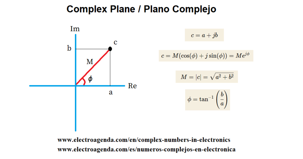
Analyzing the graph, it becomes clear that the operator j implies a 90º counterclockwise phase shift. So that both parts, real and imaginary, are orthogonal because the axes on which they are located form an angle of 90º.
1.4.2 Equivalent Expressions
From the above graph, using basic trigonometry, it can be deduced that the complex number c is equal to:
\begin{equation} c = M(\cos(\phi)+j\sin(\phi))=Me^{j\phi} \end{equation}
Where M is the modulus of the complex number and ϕ represents the phase:
\begin{equation} M = |c| = \sqrt{a^2 + b^2} \end{equation}
\begin{equation} \phi = \tan^{-1}\left(\cfrac{b}{a}\right) \end{equation}
In summary, the following table shows the different ways of writing or representing the complex number c:
| Notation | Expression |
| Cartesian | \begin{equation} c = a+jb \end{equation} |
| Trigonometric | \begin{equation} c = M(\cos(\phi)+j\sin(\phi)) \end{equation} |
| Polar | \begin{equation} c = Me^{j\phi} \end{equation} |
| Module-Angle | \begin{equation} c = M\phase\phi \end{equation} |
2. Applications of Complex Numbers
The applications of complex numbers in electronics [1][2] and communications [3][4] are articulated on the basis of the phasor definition, a mathematical representation of a tone that simplifies calculations and the understanding of multiple concepts.
One of the typical applications is circuit theory [2], where the phasors allow a simple analysis of the sinusoidal steady state. Furthermore, the use of phasors can be generalized to the analysis of signals, composed of multiple tones, in any linear system. Hence the relevance of complex numbers in signal theory [3][4] and communications [6].
2.1 Phasors
A phasor is a complex number that represents a tone or sinusoid of time invariant and fixed amplitude and phase. The mathematical and graphical representation of this concept is developed below.
2.1.1 Mathematical Representation
A generic sinusoid v(t) can be defined by its angular frequency ωi, amplitude A, and phase at the time origin ϕ. (Note that ωi, A, y ϕ, are time invariant). Its notation with real numbers is:
\begin{equation} v(t) = A\cos(\omega_i t+\phi) \end{equation}
Applying the basic fundamentals of complex numbers explained above, v(t) can also be represented by the following equalities:
\begin{equation} V = Ae^{j\phi} = A\phase\phi \end{equation}
\begin{equation} v(t) = \real[Ve^{j\omega_i t}] \end{equation}
That is, given a sinusoid v(t) at a fixed angular frequency ωi, it is possible to define a complex number V, called phasor, which allows to recover the real original tone unambiguously by applying equation (21). It is observed that the real signal is obtained simply by projecting the moving phasor on the real axis.
Obviously, and here lies the potential of complex numbers in this application, it is much simpler to operate with the phasor V than with the real tone v(t). As we will see in the rest of the text, operations with phasors can be simplified and generalized to tones and signals within a system. And only at the end of the process to obtain the real output tone or signal in a simple way.
2.1.2 Graphical Representation
A phasor can be illustrated in two ways: static and dynamic, as shown in the following graph generated with MATLAB [7]:
The static representation shows a vector whose modulus and angle are determined by the amplitude A and the phase ϕ of the original sinusoid in the time origin. In the dynamic representation, the phasor is rotated at its angular frequency by adding the phase ωit. Again, the real signal is obtained as the projection of the rotating phasor on the real axis.
It is immediate to understand that the concepts illustrated in this section can be extended linearly to the operation with a larger number of independent phasors. Because of the vector dimension of the complex plane, one can operate with phasors in the same way as one operates with vectors. Thus, the addition and subtraction of phasors of the same frequency results in a phasor that uniquely represents the resulting signal.
2.2 Frequency Domain
Complex numbers facilitate the analysis of linear systems in the frequency domain. For example, a classic application of complex numbers in electronics is the theory of sinusoidal steady-state circuits [2]. In practice, the aim of this text is not to review the basic concepts of circuit theory. Therefore, generic mathematics around the associated operations will merely be shown.
The sinusoidal input of a circuit vi(t) is denoted by its associated phasor Vi such that:
\begin{equation} v_i(t) = A_i\cos(\omega_i t+\phi_i) \end{equation}
\begin{equation} V_i = A_ie^{j\phi_i} \end{equation}
The operation of the circuit is determined by linear elements: resistors, capacitors and coils. For the circuit node representing the output, a complex transfer function H(ω) can be obtained with respect to the input node such that:
\begin{equation} H(\omega)=|H(\omega)|e^{j\arg{(H(\omega))}}\end{equation}
So that the output phasor Vo at the working frequency ωi, is obtained as follows:
\begin{equation} V_o =V_i H(\omega)\Bigr|_{\omega=\omega_i}= A_i|H(\omega_i)|e^{j[\phi_i+\arg{(H(\omega_i))}]}\end{equation}
And, again, it is univocally related to the real output signal vo(t) by equation (21), such that:
\begin{equation} v_o(t) = A_i|H(\omega_i)|\cos[\omega_i t+\phi_i+\arg{(H(\omega_i))}] \end{equation}
Thus, phasors allow simplifying the operation with sinusoids in the resolution of circuits [2] or linear systems. In general, by extending the analysis to all the frequencies that compose an input signal, the output signal of the system can be extrapolated. Another alternative is to process directly in the time domain as explained below.
2.3 Time Domain
The previous example has shown what happens to a tone in a circuit [2]. But the analysis with complex numbers can be generalized to any linear system, and to all frequencies of the system, by directly analyzing the signals in the time domain. For a correct understanding of this concept it is necessary to study the Hilbert Transform [8], and two forms of complex signals associated with a real signal: the Analytic Signal and the Complex Envelope.
2.3.1 Temporal Generalization of the Fasor
A practical example to visualize the usefulness of complex numbers in linear signal processing is to analyze a constellation of data as used in communications theory [6]. Given a signal in phase i(t) and a signal in qudrature q(t), both forming a bandpass constellation [6] such that:
\begin{equation} s(t) = i(t)\cos{\left(\omega_c t \right)} + q(t)\sin{\left(\omega_c t \right)} \end{equation}
The analytic signal and the complex envelope are, respectively:
\begin{equation} s_{a}(t) = [i(t) - jq(t)]e^{j\omega_c t} \end{equation}
\begin{equation} s_{a\downarrow}(t) = [i(t) - jq(t)] \end{equation}
In addition, it holds that:
\begin{equation} s(t) = \real[s_{a}(t)] = \real[s_{a\downarrow}(t)e^{j\omega_c t}] \end{equation}
Comparing equation (30) with equations (20) and (21), it is observed that the complex envelope represents a phasor that changes over time. It is thus confirmed that the analytic signals allow us to generalize complex analysis beyond phasors, extending it to any temporal signal.
2.3.2 Graphical Example
A constellation consistent with equation (27), and generated with MATLAB [7], is illustrated below:
Each symbol is represented in the complex plane dynamically over time. While the projection on the real axis of the analytic signal represents the real signal, the modulus of the complex number represents the envelope of the signal, which varies as a function of the symbol.
It is observed that the complex envelope is equivalent to the static representation of the phasor, although time-varying. Likewise, the analytic signal reproduces the dynamic representation of each phasor.
3. Complex Numbers Conclusions
The conclusions of this text are as follows:
- Complex numbers extend the real numbers by adding an imaginary part orthogonal to the real part.
- The j operator, which accompanies the imaginary part, is a mathematical element whose essence is difficult to understand. However, thanks to Euler’s formula, it can be deduced that the j operator implies a 90° counterclockwise phase shift.
- Complex numbers simplify calculations and the understanding of linear systems, as in the case of circuit theory [2], signal processing [3][4] or communications [5][6].
- The simplification mentioned in the previous point can be obtained both in the time domain and in the frequency domain.
Bibliography (Sponsored)
[1] Electronics, Allan R. Hambley.
[2] Electric Circuits, James Nilsson.
[3] Communication Systems, A. Bruce Carlson.
[4] Signals and Systems, A. V. Openheim.
[5] Understanding Digital Signal Processing, Richard Lyons.
[6] Digital Communications, Bernard Sklar.
[7] MATLAB Guide
[8] Hilbert Transform in Signal Processing, Stephan Hahn.
Subscription
If you liked this contribution, do not hesitate to subscribe to our newsletter: