Digital Electronics

3.4 Digital Electronics

Starting with the electron, and by increasing the level of abstraction, the evolution has been shown passing through voltages/currents until reaching bits, ‘1’s and’ 0’s. Digital electronics solves real problems and needs by operating only with these bits. This section summarizes the basic theory of digital circuits and presents the higher-level devices that arise from it, specifically programmable logic and microprocessors and microcontrollers.

3.4.1 Digital Circuits Fundamentals

As explained, analog electronics is built on fundamental laws that apply to any distribution of active and passive components, so that voltages/currents can be calculated at any node/branch of a circuit. Similarly, digital electronics are divided into components and laws that allow knowing the binary state (‘1’ or ‘0’) at any point in the digital circuit.

The fundamental theory that defines these components and this binary or digital behavior is Boolean Algebra. Additionally, the time dimension of digital signals is realized by adding components that allow an evolution based on cycles. Finally, each of the Boolean building blocks are implemented in an analog way with transistors, allowing real digital circuits to be built. All the concepts mentioned in this paragraph are explained below.

3.4.1.1 Boolean Algebra

The digital components are called logic gates. They are elements that have any number of binary inputs and any number of binary outputs, which are a function of the inputs. Table 4 shows the most fundamental logic gates, for the case of one or two inputs and one output. Any gate with another number of inputs and outputs could be extrapolated or achieved based on those presented. Likewise, Table 4 also details the operation or “truth table” of each gate.

Once the information has been digitized, any necessary operation (multiplication, addition, subtraction, division, delay, etc.) can be carried out with a more or less complicated combination of logic gates. In this way any processing can be performed with digital operations.

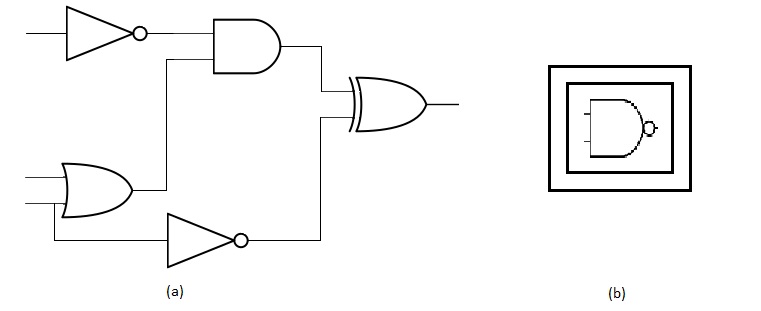
Without losing generality, Figure 8(a) shows an example of a digital circuit. From now on, and to continue with the explanations of the text, a generic digital circuit composed of any combination of logic gates will be represented as in Figure 8(b).

3.4.1.2 Switching Frequency

Up to this point it has become clear that any digital circuit is or can be made up of multiple logic gates. Every time one of the inputs to the circuit changes or switches (from ‘1’ to ‘0’ or from ‘0’ to ‘1’), the output or outputs will respond to the change according to the truth table of said complete circuit. If an output has to switch, this change will be visible in the output once the change in input has propagated through all logic gates. The more levels there are in a digital circuit, the longer it takes to wait for a switching on the inputs to take effect on the outputs.

However, many applications require meeting timing criteria that would not allow the digital circuit to wait to propagate a switch from an input to the output. Besides, in any complex applications, there may be multiple digital circuits, related or not to each other, that cannot work asynchronously, so that a clock that marks the times is necessary, a kind of conductor that establishes synchronization between all of the parts.

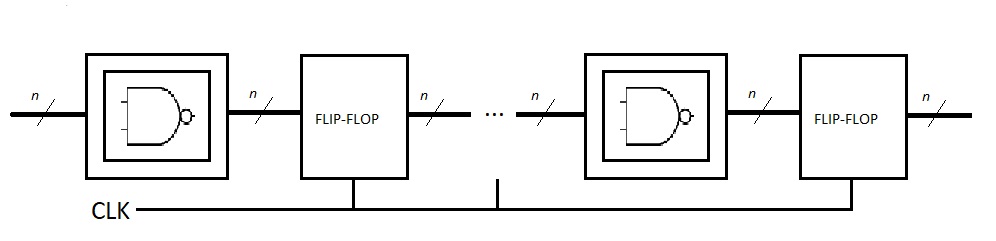
In practice, synchronization is achieved by adding a fundamental element called “flip-flop” (which can also be implemented with logic gates). The digital circuits are divided into multiple sections between flip-flops as shown in Figure 9. Every time the clock (CLK in the image) marks the start of a new cycle, the flip-flop puts the value of the bit of its input into the output, and keeps it constant until the new cycle change marked by the clock. Obviously, during the cycle time it is necessary that all digital circuits are capable of propagating their changes from input to output. In fact the minimum cycle time will be determined by the slowest circuit. Note that, without losing generality, Figure 9 considers a number n of inputs and outputs at all levels.

The cycle time of a digital circuit determines the switching frequency, which is the number of times the circuit switches per second. The higher the switching frequency, the higher the processing speed and the higher the computing power of the digital application.

3.4.1.3 Physical Implementation

The logic gates shown so far are conceptual and theoretical components, in the same way that pure ‘1’s and’ 0’s are also theoretical concepts. In analogy with what was explained for Figure 3(b), any logic gate can be implemented with transistors. The voltages/currents at the input/output of said transistors are interpreted as ‘1’s and ‘0’s depending on a threshold, as explained in section 3.3.

The relevance of the transistor implementation is that, using the right technologies, logic gates only consume power during switching between states, not all the time. This allows the creation of circuits made up of millions of transistors and working at high frequencies. In these cases we refer to specific integrated circuits where, apart from the digital design, pure analog design is also required for the optimal implementation of the logic gates, and even physical design at a very low level, as explained in section 3.1, to obtain the highest possible degree of integration.

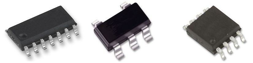
In some cases it is necessary to make simpler digital designs, whether or not they are part of more complex designs or devices. For these cases, discrete transistors can be used directly, together with components such as those shown in section 3.2.2. Discrete logic gates can also be used. These are typically supplied in common simple IC packages, as shown in Figure 10. For these types of digital designs, apart from the ‘1’s and’ 0’s, it is also necessary to consider purely “analog” issues and the timing between gates to meet the requirements of each component and its interfaces. In contrast, the devices discussed in the following sections allow you to almost completely abstract from analog issues and design at the digital level, thinking purely in bits or even at a higher level.

Bibliography (Sponsored)
[1] Digital Fundamentals, Thomas Floyd

---

<= Mixed Signal Electronics

Advanced Digital Devices =>

---

Subscription
If you liked this contribution, feel free to subscribe to our newsletter: