The complex envelope is a baseband analytic signal. It is obtained by suppressing the negative (or positive) frequencies of a real bandpass signal, and transferring the remaining spectral content to baseband. Due to the complex notation and the spectral efficiency of the resulting signal, the complex envelope is very useful in both linear system simulation and real-time digital signal processing.
The above concepts are explained in depth in this text, focusing mainly on the implementation of the complex envelope. The text is organized with the following table of contents:
1. Complex Envelope Definition
This section describes the spectral representation and the fundamental mathematics of a real bandpass signal and its corresponding complex envelope. For a correct understanding of the text it is recommended to review the following links on The Hilbert Transform and The Analytic Signal.
1.1 Spectral Representation
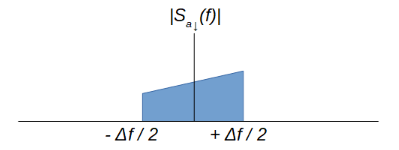
The following image shows the spectra of a real bandpass signal and its corresponding complex envelope:

Spectrally, the complex envelope is obtained by transferring the positive frequencies to baseband, and suppressing the original negative spectral content. While the original signal is real and therefore hermitic, the resulting signal does not comply with the principles of hermiticity, confirming that it is a complex signal.
Graphically, the bandwidth of the complex envelope is half that of the original signal. Therefore, according to the Nyquist criterion, the complex envelope can be sampled at half the rate of the bandpass signal.
Finally, it should be noted that this text shows the complex envelope obtained from the positive frequencies. However, it is possible to do the equivalent processing with the negative frequency components, as shown in the following link.
1.2 Mathematical Demonstration
This section shows the mathematical processing to obtain the complex envelope from the real bandpass signal. Likewise, the complementary procedure that obtains a real bandpass signal from its associated complex envelope is analyzed. The case in which the real bandpass signal is defined in terms of its in-phase and quadrature components, very useful for the mathematical analysis of communications signals, is also developed.
1.2.1 Generic Signal
Let s(t) be a generic real bandpass signal. Its Hilbert transform is given by \footnotesize \hat{s}(t) [1]. The analytic signal sa(t), in which the negative frequencies have been suppressed, is obtained as follows:
\begin{equation} s_{a}(t) = s(t)+j\hat{s}(t) \end{equation}
The demonstration that the spectrum of the analytic signal, Sa(f), does not contain the negative spectral content of s(t) is almost immediate:
\begin{equation} S_a(f) = \begin{cases}S(f)+j[-jS(f)] =2S(f)&\text{for } f >0 \\ S(f)+j0 =S(f)&\text{for } f =0 \\ S(f)+j[jS(f)]=0 &\text{for } f<0 \end{cases} \end{equation}
From the analytic signal, the baseband equivalent is obtained by transferring the remaining positive frequencies to baseband. In order not to generate other replicas, it is necessary to multiply the analytic signal by the phasor located at the center or carrier frequency [2]. Thus, the complex envelope is obtained as follows:
\begin{equation} s_{a\downarrow}(t) = s_{a}(t)e^{-j\omega_c t} \end{equation}
Finally, given a complex envelope, its associated bandpass real signal is obtained by performing the inverse process that follows from equations (1) and (3):
\begin{equation} s(t) = \real[s_{a}(t)] = \real[s_{a\downarrow}(t)e^{j\omega_c t}] \end{equation}
1.2.2 Phase and Quadrature Signals
It is of special mathematical and conceptual interest to develop the above mathematical procedure starting from a generic signal s(t) expressed as a function of its components in phase, i(t), and quadrature, q(t). That is to say:
\begin{equation} s(t) = i(t)\cos{\left(\omega_c t \right)} + q(t)\sin{\left(\omega_c t \right)} \end{equation}
Applying (1) and (3) in (5), as shown in this link, the associated complex envelope is obtained:
\begin{equation} s_{a\downarrow}(t) = [i(t) - jq(t)] \end{equation}
Therefore, any implementation of the complex envelope from s(t) must give rise to the result obtained in (6).
2. Complex Envelope Implementation
The complex envelope is very useful in signal processing and linear systems [2][3], as shown in this link. Due to the complex nature of the signal, its electronic implementation [4][5][6] always has a strictly digital part associated with it. Although the input and/or output of the overall system may be analog.
The implementation of the complex envelope can be done at various levels, partially or completely covering a system. For example, the complex envelope could be used for the following functions:
- Processing of an incoming signal, as in the demodulator of a receiver.
- Generation of an outgoing signal, as in a transmitter modulator.
- Regeneration and/or modification of a signal: involves the combination of the two previous points.
This section analyzes the implementation of the complex envelope both at a purely analytical and simulation level, as well as for real-time systems.
2.1 Simulated Time Processing
The implementation of the complex envelope to simulate a system is derived directly from the equations shown in section 1.2. The signals generated as the source of the simulation must follow the structure of equation (6), in its digital version:
\begin{equation} s_{a\downarrow}(n) = s_{a\downarrow}(n't_s) = [i(n't_s) - jq(n't_s)] = [i(n) - jq(n)] \end{equation}
Where n’ and ts represent the sample number and sampling time respectively. For simplicity, in the rest of the text the variable n will be used, which is equal to the product of n’ and ts. Although in practice n=t, for the sake of clarity t will be used as the independent variable in analog signals, and n in the case of discrete signals.
All elements of the simulated system, whether baseband or bandpass, must be implemented with their digital complex envelope associated with the center frequency of the particular element. For example, the transfer function of a real bandpass filter must be translated in frequency to obtain its complex envelope.
In this way, the simulation of the system allows obtaining the signal in any part of the chain. The real bandpass signal associated to each complex envelope would be obtained with equation (4) in its digital version:
\begin{equation} s(n) = \real[s_{a\downarrow}(n)e^{j\omega_c n}] \end{equation}
This is the simulation method used in system simulators such as SystemVue, QucsStudio o MATLAB/Octave [7]. For example, the simulation below was performed with the latter. It generates a digital quadrature modulation where the duration of each symbol coincides with a period of the carrier:
2.2 Real Time Processing
In real-time systems, once the complex envelope is available, all the ideas explained in section 2.1 apply equally. Furthermore, in this case it is necessary to ensure that all digital mathematical operations, such as filtering, must comply with the timing associated with the sampling frequency of the signal. Therefore, the technology selected for processing (ASIC, uC or FPGA) must be able to support the required operation speed.
An essential difficulty of real-time systems is the transition from the bandpass signal, typically analog, to the complex envelope and vice versa. This section shows several schemes to perform this process, and they are classified according to the number of analog-to-digital converters -ADC- (or digital-to-analog -DAC-) used in the implementation.
2.2.1 Bandpass Signal => Complex Envelope
The following describes how to obtain the complex envelope from the real bandpass signal using one or two ADCs. In all cases the advantages and disadvantages of each implementation are listed.
2.2.1.1 Implementation with 1 ADC
The following scheme allows to obtain the complex envelope from the real bandpass signal using an ADC:

First, the bandpass signal must be sampled directly. Then, once the signal has been digitized, it must be mixed with a phasor centered on the carrier frequency to be transferred to baseband. Finally, a last low pass filter (LPF) removes the unwanted replicas.
Note that, for simplicity, in the image above the sampling is performed in the first Nyquist zone. But it is also possible to sample in other Nyquist zones, so that the center frequency of the digitized signal may not coincide with that of the analog signal.
The complex signal is obtained just after multiplication by the phasor for the frequency translation. Up to this point, the imaginary part of the digital signal is equal to zero. In practice, this translation can be implemented using several strategies:
- If multipliers are not available in the physical digital device, algorithms such as CORDIC can be used.
- If the technology used has sufficiently fast multipliers, it can be used an NCO and a mechanism that obtains the sine and cosine samples needed to generate the phasor. Typically, memories would be used to store fixed sine/cosine samples, and potentially interpolators to calculate intermediate samples and increase accuracy.
The main advantage of this implementation is that it requires only one ADC. However, the associated disadvantage is that the sampling frequency of the ADC must be at least twice that required by the complex envelope. This is because it samples the bandpass signal directly instead of a baseband signal.
2.2.1.2 Implementation with 2 ADCs
By converting the real bandpass signal to baseband in a first step, the required sampling frequency can be minimized. Consequently, the power consumption associated with the conversion could be reduced. However, this scheme has the disadvantage of requiring 2 ADCs, as shown in the following image:

The mathematical justification for this implementation is given below. Let s(t) be the signal defined in equation (5). After multiplying by the in-phase and quadrature sinusoids respectively, it is obtained that:
\begin{equation} s_i(t) = 2i(t)\cos^2{\left(\omega_c t \right)} + 2q(t)\sin{\left(\omega_c t \right)}\cos{\left(\omega_c t \right)} \end{equation}
\begin{equation} s_q(t) = 2i(t)\cos{\left(\omega_c t \right)}\sin{\left(\omega_c t \right)} + 2q(t)\sin^2{\left(\omega_c t \right)} \end{equation}
After applying the following trigonometric equalities:
\begin{equation} \cos^2{\left(\omega_c t \right)} = \cfrac{1}{2} +\cfrac{\cos{\left(2\omega_c t \right)}}{2} \end{equation}
\begin{equation} \sin{\left(\omega_c t \right)}\cos{\left(\omega_c t \right)} = \cfrac{\sin{\left(2\omega_c t \right)}}{2} \end{equation}
\begin{equation} \sin^2{\left(\omega_c t \right)} = \cfrac{1}{2} -\cfrac{\cos{\left(2\omega_c t \right)}}{2} \end{equation}
It follows that:
\begin{equation} s_i(t) = i(t) + i(t)\cos{\left(2\omega_c t \right)} + q(t)\sin{\left(2\omega_c t \right)} \end{equation}
\begin{equation} s_q(t) = i(t)\sin{\left(2\omega_c t \right)} + q(t) - q(t)\cos{\left(2\omega_c t \right)} \end{equation}
If the in-phase and quadrature components, i(t) and q(t), are band-limited, and the carrier frequency is sufficiently high, at the output of the low pass filters (LPF) it is obtained that:
\begin{equation} s_i(t) \xRightarrow{LPF} i(t) \end{equation}
\begin{equation} s_q(t) \xRightarrow{LPF} q(t) \end{equation}
Therefore, the original in-phase and quadrature components would have been recovered. Finally, the sequence that is processed discretely is [i(n)–jq(n)] as shown in equation (7).
Note that this demonstration relies on the calculations presented in section 1.2.2 to derive equation (6). But it is also possible to perform an exclusively graphic demonstration starting from the original bandpass spectrum [8].
2.2.2 Complex Envelope => Bandpass Signal
The transition from the complex envelope to its associated real bandpass signal can be performed with schemes complementary to those described in the previous section.
2.2.2.1 Implementation with 1 DAC
The implementation with 1 DAC is carried out with the following scheme:

From the complex envelope the in-phase and quadrature components can be separated. Both signals are upconverted in frequency in a completely digital way, with techniques equivalent to those explained in section 2.2.1.1. Finally, a DAC plus a filter that eliminates unwanted replicas allows the recovery of the associated real bandpass signal.
Equivalently, the advantage of this strategy is that only one converter is needed. However, the main disadvantage is that the working sampling frequency is not optimal, since it operates with bandpass signals in the discrete domain.
2.2.2.2 Implementation with 2 DACs
The implementation with 2 DACs is carried out with the following scheme:

In this case, from the complex envelope, the in-phase and quadrature baseband components are generated. Then, using two DACs, the corresponding analog signals are obtained. Finally, the high frequency conversion is also performed in the analog domain.
The advantages and disadvantages are those corresponding to the equivalent scheme described in section 2.2.1.2. The sampling frequency used in the discrete domain is the lowest possible, since it operates with baseband signals. On the other hand, it is necessary to use two DACs.
3. Complex Envelope Conclusions
The main conclusions of the text on the complex envelope are as follows:
- The complex envelope is a baseband analytic signal associated with a real bandpass signal.
- It is obtained by suppressing the negative frequencies of the original signal and transferring the positive frequencies to baseband.
- The main advantages of the complex envelope are those associated with complex notation (separation of in-phase and quadrature components; and ease of obtaining instantaneous amplitude and phase of the signal) and spectral efficiency (processing of the spectrum of interest without overlapping or duplicated frequency components).
- It is very useful in signal and system processing, both in simulated and real-time implementations.
- In real-time systems, the complex envelope can be obtained from the bandpass signal using 1 or 2 ADCs. Equivalently, the step from a complex envelope to the associated real bandpass signal can be performed with 1 or 2 DACs.
- Implementations with 1 converter have the disadvantage of using a sampling frequency at least twice the theoretical minimum, which is obtained in implementations with 2 converters.
- Implementations with 2 converters use more resources, but minimize the sampling frequency and, potentially, the power consumed in the conversion.
Bibliography
[1] Hilbert Transform in Signal Processing, Stephan Hahn.
[2] Communication Systems, A. Bruce Carlson.
[3] Signals and Systems, A. V. Openheim.
[4] Electric Circuits, James Nilsson.
[5] Electronics, Allan R. Hambley.
[6] Electronic Principles, A. Malvino.
[7] MATLAB Guide
[8] Understanding Digital Signal Processing, Richard Lyons.
[9] Signal Processing Courses
Subscription
If you liked this contribution, feel free to subscribe to our newsletter: