
The analytic signal is a complex representation of a real signal, obtained by suppressing the negative frequency components of the original signal. From the analytic signal is derived the equivalent baseband signal, also an analytic representation known as complex envelope. Both representations are used in signal processing techniques due to their main advantages: spectral efficiency and the ability to obtain the instantaneous envelope and phase of a signal.
The text is organized with the following contents. First, the analytic signal and the complex envelope are defined, both mathematically and graphically. Next, the applications of both representations are reviewed, explaining their main advantages. Finally, the fundamental conclusions of the text are derived. Overall, the table of contents is as follows:
1. Analytic Signal Definition
In this section the analytic signal and the complex envelope are defined both graphically and mathematically. For a correct understanding of the text it is recommended to review the Hilbert Transform, explained in detail in this link.
1.1 Spectral Representation
The following image shows the spectrum of a generic real bandpass signal s(t), and the spectra of their corresponding associated complex representations: analytic signal sa(t) and complex envelope sa↓(t).
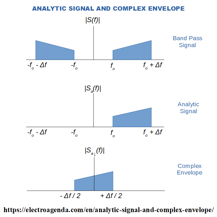
It is observed that in the analytic signal sa(t) the negative frequency components have been suppressed. On the other hand, the complex envelope sa↓(t) is obtained by a frequency translation of sa(t) to become a baseband representation.
While the spectrum of the original signal is hermitic, since it is obtained from a real signal [1] [2], the spectra of complex analytic signals do not exhibit hermiticity. In other words, the module of the spectra of analytic signals are not symmetric about zero.
Finally, it is also possible to obtain the analytic signals corresponding to the negative frequencies, suppressing the positive ones. For this it is necessary to start from the conjugated analytic signal, as detailed in this link.
1.2 Mathematical Proof
1.2.1 Bandpass Analytic Signal
Given a real bandpass signal s(t), the analytic signal is obtained by means of the following equation:
\begin{equation} s_{a}(t) = s(t)+j\hat{s}(t) \end{equation}
Where \footnotesize \hat{s}(t) represents the Hilbert Transform of s(t) [3].
In addition, as will be shown below, the conjugate variant of the analytic signal also exhibits relevant properties:
\begin{equation} s_{a}^*(t) = s(t)-j\hat{s}(t) \end{equation}
It is practically immediate to prove that in the analytic signal sa(t) negative frequencies have been removed from the original signal:
\begin{equation} S_a(f) = \begin{cases}S(f)+j[-jS(f)] =2S(f)&\text{for } f >0 \\ S(f)+j0 =S(f)&\text{for } f =0 \\ S(f)+j[jS(f)]=0 &\text{for } f<0 \end{cases} \end{equation}
Likewise, in the case of the conjugated analytic signal, the positive frequencies have been eliminated:
\begin{equation} S_a^*(f) = \begin{cases}0&\text{for } f >0 \\ S(f)&\text{for } f =0 \\ 2S(f) &\text{for } f<0 \end{cases} \end{equation}
Although not very intuitive, from the analytic signal, defined in (1) and (2), the original signal including its suppressed frequencies can be recovered by simply taking the real part of the signal:
\begin{equation} s(t) = \Re{[s_{a}(t)]} = \Re{[s_{a}^*(t)]} \end{equation}
This last property is very relevant. It implies that the processing of linear systems [1] [2] can be performed with the analytic representations of the signals and filters involved. Simply taking the real part of the resulting signal is enough to obtain the same result as would have been obtained with the original signals and filters.
1.2.2 Baseband Complex Envelope
As illustrated in the image above, the complex envelope is obtained by translating the analytic signal from its center frequency to DC. In order to translate the spectrum in this way, without creating additional replicas, it is necessary to multiply its signal in the time domain by the phasor located at the center frequency ωc [1] such that:
\begin{equation} s_{a\downarrow}(t) = s_{a}(t)e^{-j\omega_c t} \end{equation}
\begin{equation} s_{a\uparrow}(t) = s_{a}^*(t)e^{j\omega_c t} \end{equation}
Recovering the original signal from the complex envelope is more complicated, because another frequency translation is required:
\begin{equation} s(t) = \real[s_{a}(t)] = \real[s_{a\downarrow}(t)e^{j\omega_c t}] \end{equation}
\begin{equation} s(t) = \real[s_{a}^*(t)] = \real[s_{a\uparrow}(t)e^{-j\omega_c t}] \end{equation}
This last property is also very relevant in digital signal processing. In linear systems [1] [2] all calculations can be performed using the baseband analytic variants of the signals and filters involved. Subsequently, the resulting bandpass signal would be obtained by translating back to the center frequency and taking the real part.
2. Envelope and Phase
In general, the analytic signal provides all the advantages associated with the complex plane representation. This is especially noticeable when dealing with modulations, demodulations and communications signals.
This section demonstrates both mathematically and with graphical examples an important property associated with complex notation and, consequently, with the analytic signal. More specifically, the complex representation has the inherent ability to easily discern the instantaneous envelope and phase of a real bandpass signal. Also the power since it is directly related to the envelope. In the following, this property is particularized individually for both the analytic signal and the complex envelope. In addition, a video illustrating this processing with a realistic example is shown.
2.1 Analytic Signal
First, starting from the bandpass analytic signal of equation (1), it is written as a function of its module and phase:
\begin{equation} s_{a}(t) = |s_{a}(t)|e^{j [\arg(s_{a}(t))]} \end{equation}
Where:
\begin{equation} |s_{a}(t)| = \sqrt{s^2(t)+\hat{s}^2(t)} \end{equation}
\begin{equation}\arg(s_{a}(t)) = \arctan{\left(\frac{\hat{s}(t)}{s(t)}\right)}\end{equation}
From the property of equation (5), and developing Euler’s formula in (10), it follows that:
\begin{equation} s(t) = |s_{a}(t)|\cos{\left[\arg(s_{a}(t))\right]} \end{equation}
Therefore, it has been demonstrated that the instantaneous envelope and phase of the signal s(t) are equal respectively to the module and phase of the analytic signal sa(t).
2.2 Complex Envelope
Next, the equivalent envelope and phase calculations of s(t) are performed from the complex envelope.
First, it is desired to obtain the complex envelope in terms of its module and phase:
\begin{equation} s_{a\downarrow}(t) = |s_{a\downarrow}(t)|e^{j [\arg(s_{a\downarrow}(t))]} \end{equation}
From equation (6), replacing the analytic signal with the result obtained in (10), it is deduced that:
\begin{equation} s_{a\downarrow}(t) = |s_{a}(t)|e^{j [\arg(s_{a}(t))]}e^{-j\omega_c t} \end{equation}
Where, comparing (14) and (15), it is obtained that:
\begin{equation} |s_{a\downarrow}(t)| = |s_{a}(t)| \end{equation}
\begin{equation}\arg(s_{a\downarrow}(t)) = -\omega_c t + \arg(s_{a}(t)) \end{equation}
Since the envelopes of the analytic signal and the complex envelope are the same, the only difference is in the phase. Developing (13) with the result of (17) it is obtained that:
\begin{equation} s(t) = |s_{a\downarrow}(t)|\cos{\left[\omega_c t +\arg(s_{a\downarrow}(t))\right]} \end{equation}
Therefore, comparing (13) and (18) it is observed that unlike the complex envelope, the phase of the analytic signal includes the carrier. In other words, the complex envelope incorporates the baseband version of the instantaneous phase of the original signal.
2.3 Practical Example
In this section, the above conclusions are generalized to the practical case of quadrature modulations. A moving example is also shown to illustrate the envelope and phase evolution of both analytic signals within the modulation.
2.3.1 Quadrature modulation
Given two baseband signals i(t) and q(t), modulating a carrier in phase and quadrature respectively, the original bandpass signal is obtained as:
\begin{equation} s(t) = i(t)\cos{\left(\omega_c t \right)} + q(t)\sin{\left(\omega_c t \right)} \end{equation}
Its Hilbert Transform is:
\begin{equation} \hat{s}(t) = i(t)\sin{\left(\omega_c t \right)} - q(t)\cos{\left(\omega_c t \right)} \end{equation}
The associated analytic signal is obtained with equation (1) and, after performing several manipulations and solving Euler’s formula, it follows that:
\begin{equation} s_{a}(t) = [i(t) - jq(t)]e^{j\omega_c t} \end{equation}
Finally, the associated complex envelope, defined in (6), produces the following result:
\begin{equation} s_{a\downarrow}(t) = [i(t) - jq(t)] \end{equation}
It can be seen that the analytic signal and complex envelope are bandpass and baseband representations of the original signal in the complex plane. Note also that the 180º phase shift associated to the signal q(t) is not relevant, since the recovery of the original signal with (5) or (8) is independent of this phase shift.
2.3.2 Moving Constellation
The following video shows an example of a quadrature bandpass signal and its complex analytic representations. For simplicity, and without loss of generality, the period of the carrier is equal to the duration of a symbol.
The above deductions can be observed graphically. First, the module of the analytic signals coincides with the envelope of the bandpass signal. Also, the phase of the analytic signal is equivalent to the phase of the bandpass signal. Finally, the complex envelope is just a baseband representation, which can be viewed as a sophisticated phasor since its instantaneous envelope and phase evolve with time.
3. Linear Systems Processing
The analytic signal is a spectrally efficient representation of a real bandpass signal. This property arises from the elimination of frequencies that can be considered superfluous due to the hermetic symmetry of the spectrum of a real signal. How this property translates into advantages for the processing of linear systems is explained didactically below.
3.1 Real Signal Processing
We start from a linear LTI system where si(t) represents the input signal and so(t) represents the output signal. The behavior of the system is defined by its impulse response h(t). With the previous data, the signal processing of the system can be represented in the frequency domain. As an example, the following spectra are used:

For the conventional application with real signals, hermitically symmetric spectra are obtained. Note that the images of the spectra show only the modules and not the phases for simplicity.
3.2 Analytic Signal Processing
In theoretical and practical terms, signal processing of a linear system can also be performed with analytic variants of real signals and filters. In this regard, it is important to emphasize that the analytic representation of the filter that describes the system, ha(t), is sometimes referred to as a quadrature filter.
As illustrated in the image above, the equivalent spectral processing would consist of employing only the positive spectra (or only the negative spectra, although that strategy is not shown in the example). Note that the same result would be obtained starting from si(t) in its real version, or even using si(t) in its analytic version and the filter h(t) in its real version.
Either way the resulting signal so(t) is the same as that obtained with real signal processing. For this, in a last step, equation (5) adapted to this case must be applied again:
\begin{equation} s_o(t) = \real[s_{oa}(t)] \end{equation}
The strategy shown in this section is typically used in theoretical developments in signal processing, such as linear circuit theory [4]. However, this strategy is not effective for real-time signal processing. In practice it requires two signal data streams (real and imaginary) with high bandwidth and sampling frequency, since bandpass signals are used. This issue is solved by using the complex envelope, as detailed below.
3.3 Complex Envelope Processing
As shown in this section, the processing of linear systems using the complex envelope allows simultaneous achievement of important advantages.
First, the original bandpass spectrum can be processed without the penalty associated with a conversion to a real baseband signal. Secondly, the processing can be performed with the sampling rate corresponding to a baseband signal, lower than that of the bandpass signal. Finally, all the advantages associated with complex notation are obtained, as explained in section 2.
From the concepts explained in this section, it can be derived the relevance of the complex envelope in digital signal processing (DSP) techniques [5] for any final application. A particularly relevant case is DSP in real-time applications. Note that this section shows these concepts in a theoretical way. More details on the practical implementation of the complex envelope are provided in this link.
3.3.1 Bandpass to Baseband Conversion
The real conversion of a bandpass signal to baseband involves a significant penalty. Due to the hermiticity of the signal, the negative and positive spectra overlap in the conversion. This effect is illustrated in the following image.

It is clear that the overlapping prevents the recovery of the original bandpass spectrum that was intended to be processed. However, by using the complex envelope, a representation of the real bandpass spectrum without overlapping is obtained.
3.3.2 Lower Sampling Rate
The next step is to adapt the processing shown above with real and/or analytic signals. The following image shows the complete equivalent scheme implemented using the complex envelope:

When processing the system with the complex envelope, a baseband spectrum signal, the data can be sampled at a lower rate. If the original bandpass signal has a bandwidth of B Hz (B=Δf in the figure), its minimum sampling rate will be equal to 2B Hz (assuming an implicit frequency conversion). However, by using the complex envelope, each of the data strings (real and imaginary) has a bandwidth of B/2 Hz and, therefore, its sampling frequency can be reduced to B Hz.
3.3.3 Resulting Band Pass Signal
Once the system processing is finished, the equivalent real bandpass signal is obtained by adapting equation (8) to this case:
\begin{equation} s_o(t) = \real[s_{oa\downarrow}(t)e^{j\omega_c t}] \end{equation}
Obviously, this step is only necessary when the linear system requires a real bandpass output. There are many applications, such as a demodulator, where processing of the complex envelope does not involve further reconstruction. Also, in some cases, non-linear processing of the analytic signal and the complex envelope can also be applied.
4. Analytic Signal Summary
The main conclusions on the analytic signal are as follows:
- The analytic signal, including the complex envelope, is a complex representation associated with a real signal.
- Given a real signal, its associated analytic signal is a spectrally efficient representation because the negative and superfluous frequencies of the original signal are suppressed.
- The complex envelope is the baseband representation of the analytic signal.
- Mathematically, analytic signals are obtained from the original real signal and its Hilbert Transform.
- The real part of the analytic signal allows the recovery of the associated original signal. In the case of the complex envelope, it is necessary to perform a complex frequency translation beforehand.
- The analytic signal allows to obtain the instantaneous envelope and phase of the original bandpass signal.
- The processing of linear LTI systems can be simplified by using the analytic signal versions.
- The complex envelope allows the processing of an originally bandpass spectrum while simultaneously reducing the sampling frequency. It is therefore a fundamental concept in DSP. [5].
Bibliografía
[1] Communication Systems, A. Bruce Carlson.
[2] Signals and Systems, A. V. Openheim.
[3] Hilbert Transform in Signal Processing, Stephan Hahn.
[4] Electric Circuits, James Nilsson.
[5] Understanding Digital Signal Processing, Richard Lyons.
[6] Signal Processing Courses
Subscription
If you liked this contribution, feel free to subscribe to our newsletter: